고정 헤더 영역
상세 컨텐츠
본문
1. 필요한 모듈 불러오기
import numpy as np
import matplotlib.pyplot as plt

import torch
import torch.nn as nn
import torch.nn.functional as F
from torchvision import transforms, datasets
2. GPU 사용가능 여부 확인
if torch.cuda.is_available() :
  DEVICE = torch.device('cuda')
else :
  DEVICE = torch.device('cpu')

print('Using PyTorch version :', torch.__version__, ' Device :', DEVICE)
3. 데이터 불러오기
BATCH_SIZE = 32
EPOCHS = 10

train_dataset = datasets.MNIST(root = "../data/MNIST",
                               train = True,
                               download = True,
                               transform = transforms.ToTensor())
test_dataset = datasets.MNIST(root = "../data/MNIST",
                              train = False,
                              transform = transforms.ToTensor())

train_loader = torch.utils.data.DataLoader(dataset = train_dataset,
                                           batch_size = BATCH_SIZE,
                                           shuffle = True)

test_loader = torch.utils.data.DataLoader(dataset = test_dataset,
                                          batch_size = BATCH_SIZE,
                                          shuffle = False)
4. 데이터 확인 및 시각화
- 데이터 size 및 type 확인
for (X_train, y_train) in train_loader :
  print('X_train :', X_train.size(), 'type :', X_train.type())
  print('y_train :', y_train.size(), 'type :', y_train.type())
  break

#X_train : torch.Size([32, 1, 28, 28]) type : torch.FloatTensor
#y_train : torch.Size([32]) type : torch.LongTensor
- 이미지 확인
plt.figure(figsize = (10, 1))
for i in range(10):
  plt.subplot(1, 10, i + 1)
  plt.axis('off')
  plt.imshow(X_train[i, :, :, :].numpy().reshape(28, 28), cmap = "gray_r")
  plt.title('Class: ' + str(y_train[i].item()))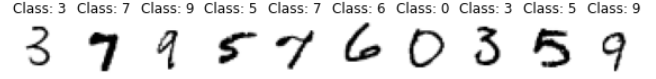
5. 모델링
- MLP 모델 설계
class Net(nn.Module):
  def __init__(self):
    super(Net, self).__init__()
    self.fc1 = nn.Linear(28 * 28, 512)
    self.fc2 = nn.Linear(512, 256)
    self.fc3 = nn.Linear(256, 10)
    self.dropout_prob = 0.5
    self.batch_norm1 = nn.BatchNorm1d(512)
    self.batch_norm2 = nn.BatchNorm1d(256)

  def forward(self, x):
    x = x.view(-1, 28 * 28)
    x = self.fc1(x)
    x = self.batch_norm1(x)
    x = F.relu(x)
    x = F.dropout(x, training = self.training, p = self.dropout_prob)
    x = self.fc2(x)
    x = self.batch_norm2(x)
    x = F.relu(x)
    x = F.dropout(x, training = self.training, p = self.dropout_prob)
    x = self.fc3(x)
    return x
- Optimizer, He-initialization 적용
import torch.nn.init as init
def weight_init(m):
  if isinstance(m, nn.Linear):
    init.kaiming_uniform_(m.weight.data)

model = Net().to(DEVICE)
model.apply(weight_init)
optimizer = torch.optim.Adam(model.parameters(), lr = 0.01)
criterion = nn.CrossEntropyLoss()

print(model)
6. 모델 학습
- train 데이터에 대한 모델 성능을 확인하는 함수 정의
def train(model, train_loader, optimizer, log_interval):
  model.train()
  for batch_idx, (image, label) in enumerate(train_loader):
    image = image.to(DEVICE)
    label = label.to(DEVICE)
    optimizer.zero_grad()
    output = model(image)
    loss = criterion(output, label)
    loss.backward()
    optimizer.step()

    if batch_idx % log_interval == 0:
      print("Train Epoch: {} [{}/{} ({:.0f}%)\tTrain Loss: {:.6f}".format(
          epoch, batch_idx * len(image), len(train_loader.dataset), 100 * batch_idx / len(train_loader),
          loss.item()
      ))
- test 데이터에 대한 모델 성능을 확인하는 함수 정의
def evaluate(model, test_loader):
  model.eval()
  test_loss = 0
  correct = 0

  with torch.no_grad():
    for image, label in test_loader :
      image = image.to(DEVICE)
      label = label.to(DEVICE)
      output = model(image)
      test_loss += criterion(output, label).item()
      prediction = output.max(1, keepdim = True)[1]
      correct += prediction.eq(label.view_as(prediction)).sum().item()

    test_loss/= len(test_loader.dataset)
    test_accuracy = 100. * correct / len(test_loader.dataset)
    return test_loss, test_accuracy
- 모델 학습
loss = []
accuracy = []
for epoch in range(1, EPOCHS + 1):
  train(model, train_loader, optimizer, log_interval = 200)
  test_loss, test_accuracy = evaluate(model, test_loader)
  loss.append(test_loss)
  accuracy.append(test_accuracy)
  print("|n[EPOCH:{}], \tTest Loss: {:.4f}, \tTest Accuracy: {:.2f} % \n".format(
      epoch, test_loss, test_accuracy
  ))
7. 결과 확인
plt.figure(figsize=(10,5))
plt.subplot(1,2,1)
plt.xlabel('Epoch')
plt.ylabel('Loss')
plt.plot(loss)
plt.subplot(1,2,2)
plt.xlabel('Epoch')
plt.ylabel('Accuracy')
plt.plot(accuracy)
plt.show()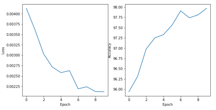
학습이 진행되면서 Loss값은 감소하고 약 98%의 정확도가 나왔다.


댓글 영역